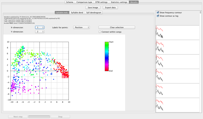
Luscinia carries out a Nonmetric Multidimensional Scaling analysis (following Kruskal’s 1964 methods) to turn the distance matrices that result from computational comparisons of sets of sounds into representations in Euclidean space.
Comparisons carried out by DTW or by Parametric methods result in a dissimilarity matrix between the compared signal units. Such matrices are not suitable for some forms of further analysis, because of the dependencies between units. Ordinating the distance matrix assigns each data-point a position in some Euclidean space. In addition, the dissimilarity measures resulting from a DTW comparison are not fully Euclidean - they do not obey the triangle inequality. This can complicate some analyses that might use a distance matrix for input, but require it to be in Euclidean space. Luscinia uses NMDS to get around this problem. In fact the series of calculations involved in producing the final ordination is as follows: (1) carry out a Principal Coordinates analysis on the distance matrix to generate initial locations for the NMDS; (2) carry out the NMDS analysis; (3) carry out a second PCO analysis that re-ordinates the data so that the maximum amount of information is found in the first Principal Coordinates. This also allows the calculation of familiar “proportion of variation explained” statistics.
On the Analysis and Visualization window, the user must set the number of dimensions for Luscinia to calculate. This is found in the Number of Dimensions for NMDS field.
The output of the analysis is a scatter plot. At the top of the window, a panel displays the summary statistics of the analysis: the proportion of variation explained by various of the dimensions, along with the stress calculated from the NMDS itself. (Values <0.1 indicate that a high proportion of the variation between signals is being explained by the ordination).
Beneath this summary information are several controls for the appearance of the scatter plot. First, X Dimension and Y Dimension allow the user to view different axes of the results on the scatter plot.
Labels for points allows the user to select how the points are color coded. Included in the drop-down menu may be the results of K-medoids and Syntactical clustering analyses, if they have been carried out. When one or other of these are available, an extra drop-down menu appears: Number of clusters, which is used to control how many clusters are shown on the scatter plot. In addition, the user can select “Population” to label points according to the population to which the individual is assigned, and “Position” for units other than songs, as shown in the figure above. Here, points are labeled according to their position within a song.
Connect within songs draws grey lines between the points for adjacent units within songs. This is an alternative simple visualization of potential syntactical dependencies.
The scatter plot itself is interactive. A user can click on a point on the screen, and Luscinia will draw a sketch spectrogram of the data-point on the right of the window. Alternatively, a user can click and drag (as shown above) and highlight a rectangular area of the scatter plot. Then Luscinia will plot sketches for all points within the highlighted area.
Clear selection clears the highlighted region from the scatter plot.
